The best player in the world according to Artificial Intelligence

It is a model that reflects the "chance" that a shot is converted into a goal. An xG model calculates for each shot the probability of scoring according to what we know: the position of the striker, the distance to the goal ... The higher the xG, 1 being the maximum, the higher the probability of scoring. 
The xG model answers the following problem: it is not enough to say that one has scored 35 goals this season, and another has scored 27 goals, to deduce that the former is better than the latter. The question remains as to the context, did the former have more attempted shots? Better dispositions? Was the second less fortunate? 
The simplest way to understand what an xG model is, is to take an example such as penalties. As a general rule, penalties are around 0.75 xG, based on the historical conversion rate. A penalty is the easiest attempt to classify, as it is an isolated situation in the game. In practice a penalty is therefore converted into a goal 75% of the time. 
Thus, the objective is to create a predictive model that for any shot, in any situation, gives us the probability that this event will lead to a goal. 
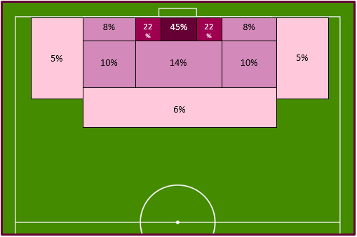
We illustrate the percentage of conversion according to the zones of the field with the diagram below :

We are looking for an indicator that, for a given shot, gives us the probability that a player will score a goal. The first thing to clarify is that we will therefore not take individual performance into account in the model. It is obvious that if Messi comes face to face with the goalkeeper, the chances of scoring a goal will be higher than with a weaker player. On the other hand, if Alisson - considered the best goalkeeper in the world - is keeping goal, then the chances of scoring could go down. But that is not the purpose of the metric. We try to normalize through our data the probability that a player will score from a certain position in a certain situation.

First of all it is important to divide our model according to the situations in which the player finds himself when taking his chance. Indeed, we are not going to use the same variables to evaluate a shot in open play and a free kick. A model must therefore be developed for each of the different situations in a match, for example : 

• During open play;
• For a penalty kick;
• For a direct free kick;
• For an indirect free kick;
• For a corner.

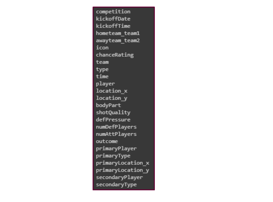
Then for each of these situations the associated model will evaluate different variables. In recent years, artificial intelligence has made it possible to collect large amounts of data automatically and to label thousands of events as a shot.  I refer you to our previous article for more details [1]. In our case the factors that influence the xG model are : 

• Location (distance, angle or area);
• The use of strong or weak foot;
• The last pass before the shot (pass, center etc);
• Possession before the attempt;
• Dribbling (just dribbled a player, just dribbled the goalie);
• The team plays away or at home;
• The team leads or loses;
• Speed of attack;
• Number of defenders;
• The pressure of the defenders (close to the shooter, between the ball and the goal).

Thus we notice that we can get a lot of information about an event such as a shot, even though it is not always easy to collect this information. This is a central issue in Football Analytics and in Data Science in general. The more data we have, the better our prediction will be. Suppliers like Opta use the latest advances techniques in artificial intelligence to acquire this digital goldmine and interest the clubs.

In this part we will develop a first model, we have some of the variables and situations exposed previously. The data comes from the former Football Analytics platform: Stratabet. More precisely, we have 26 variables for just under 30,000 shooting situations in three major European championships (Spain, England and Germany) during the 2017-2018 season. That is 1252 matches, 1350 players and 785 different strikers.

We start by looking for possible duplicates. Our dataset does not have any, but there is no column that acts as a unique identifier: we create one.
Then for each variable we look for null values, in which case, if possible, we proceed with imputation, otherwise we delete the row. Always for each parameter we use adequate statistics and visualizations to detect outliers. 
As an illustration, the variable "type" tells us whether a shot was taken in the game or from a direct free kick. Let's take a closer look :

We notice two things. First, some of the shots are in the surface. Except they are direct free kicks, which is impossible in this position, so we take them out. 
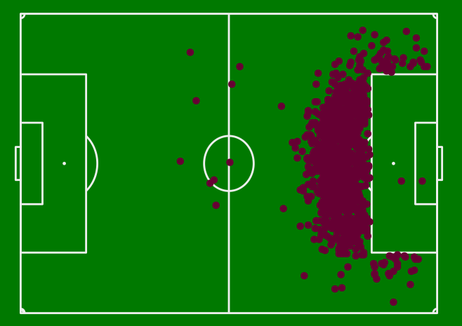
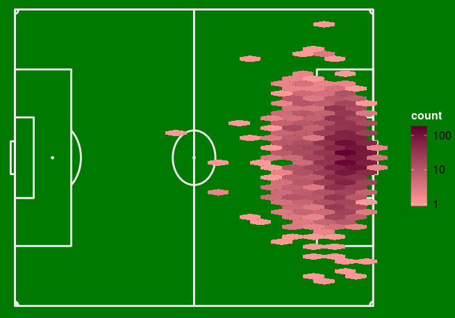
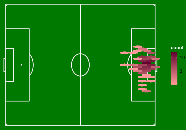
Second, some were shot from far too far away to be considered an attempt to score a goal. This may also be the case for shots in play. Let's look at the heatmap of all the attempts:

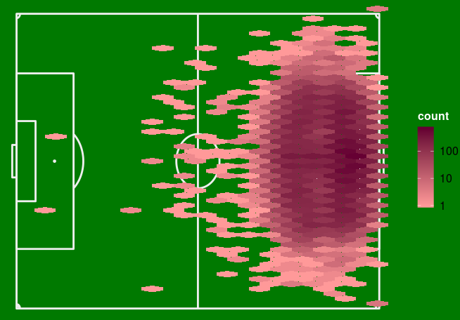
And those that led to a goal:

We then withdraw the attempted shots before the median line, considering the others as outliers.
Let's take a last example with the variable "BodyPart". As its name indicates, it allows us to know with which part of the body the player has shot. We have:

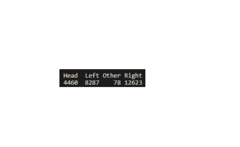
Not surprisingly, there are more right-handed players, so more right-foot shots. The problem is that our dataset does not tell us which is the strong or weak foot of the player. Knowing that he took his chance with his right or left foot doesn't give us any more information than just knowing that he shot with his right or left foot. We therefore modify this variable and get :

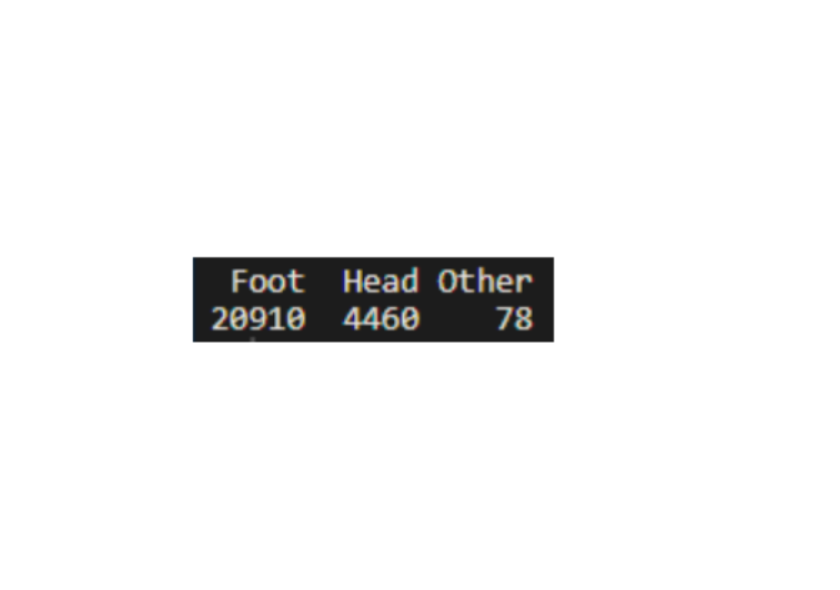
Let's look at the connection between the body part used and our target: 

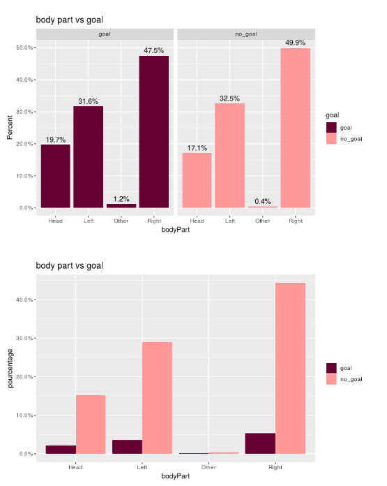
If you only consider the body part when shooting, you have 13% chance of scoring if you use your foot, 15% if you use your head and 81% if you use another part! Of course this rarely happens, but let's look at the heatmap of these shots and the passes before them:

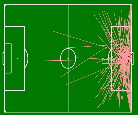
We notice that this happens almost only in the penalty area, very close to the opponent's goal and often on a centre. It is easy to imagine an action such as crossing the ball or a volley that have a great chance of being converted into a goal in view of the distance.  
Thus, with an exploratory analysis we can obviously "clean up" our data but also learn and observe certain patterns.

Another task that can bring a lot of information to our model is adding variables. For example, we can enrich our model with data from other sources such as the weak or strong foot of each player. We have not implemented this yet, since we want to create a first model from what we have and that can be complexified later on. We however calculate the distance and the angle of the shot from the location coordinates x and y. Also we introduce a psychological aspect with a variable that indicates if the player who shoots is playing at home or away and if his team leads, is tied, or loses at the moment the player takes his shot.

Once our dataset is clean, we need to select the variables to be used in our model. This step can be tricky when you have a large number of variables. Indeed, it can be difficult to apprehend the effects on the target and the correlations between the variables. In our case it is not complicated to make hypothesis about the importance of the few interesting variables. Moreover during our data visualization phase we were able to assess the link between our variables and the target. For example with the variable "numDefPlayers", which represents the number of defenders between the ball and the goal:

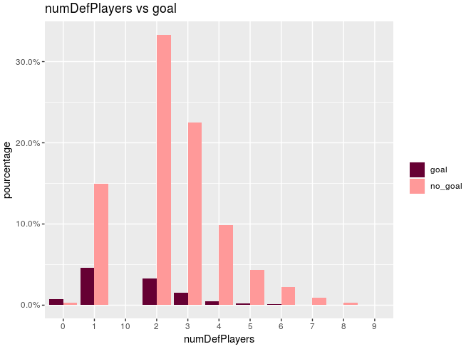
It's easy to see that the fewer defenders there are, the more shots are converted into goals. By this method we then select the variables correlated with our target: 

• chanceRating: we evaluate from 0 to 5 the ease of shooting 
• Foot: 1 if the shot was taken with the foot, 0 otherwise
• Head: 1 if the shot was taken with the head, 0 otherwise
• Other: 1 if the shot was made with another part of the body, 0 otherwise
• defPressure: the pressure exerted by the defence is estimated between 0 to 5 
• numDefPlayers: we sum the number of defenders 
• home: 1 if the shot was made at home, 0 otherwise
• away: 1 if the shot was made outside, 0 otherwise
• dist: the standard distance to the goal 
• angle: the angle of the shot on goal, 0 if you are in front, 1 if you are perpendicular.

We then develop two models. One model for the shots taken during the game and one for shots taken from a direct free kick. We have seen ealier that for penalties we can only base ourselves on historical success, which gives us 0.75 xG for each. We will thus have three models. 

In the game 

Logistic regression is a good algorithm for our first model. Indeed it is commonly implemented to estimate the probability that an instance belongs to a particular class.  It is therefore perfectly suitable for the classification of binary variables, which is our case. Moreover, it is a model that returns a probability. Indeed, let’s not forget that the purpose here is not to classify each shot, but to assess the  probability of success for each shot, and this is exactly what logistic regression will give us. Lastly, it is an interpretable model, which allows us to easily understand how the model chooses to classify the instances. 
We are also in the case of a so-called "unbalanced" dataset. That is to say that our variable to be classified is not distributed in an balanced way in our two classes.

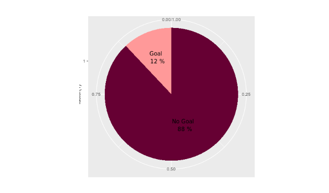
In this case, developing a model that always predicts that the shot will not hit the target will have an accuracy of 88%. First of all, we have to be careful with the metrics that we are going to chose to evaluate the performance of the model. Just observing the accuracy is not enough, especially in the case of an unbalanced dataset. We set up several metrics: precision, recall, F-score, AUC (area under curve). In addition, we perform a cross-validation to improve the reliability of the performance estimation. 
Secondly, our algorithm will have difficulty to correctly predict the under represented class of our dataset, because of the sample imbalance. We can then perform a re-sampling to counter this problem. More precisely, we apply the most commonly used methods for oversampling: Adjust class weight RL, Random over sample, SMOTE, ADASYN [2]. But also for undersampling: Adjust class weight RL, Random under sample Near miss 1 and 2, TomeksLinks, Edited nearest neighbours [3].
We get :

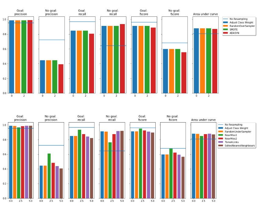
The difficulty for this type of problem is to get a good trade-off between recall and accuracy [4]. That is to say, to succeed in detecting shots that will give a goal (accuracy) and to detect enough of them (recall), knowing that when one improves, the other decreases. So if we want to detect a lot of shots (recall) we will also make mistakes more often (accuracy), we must find the right balance. We choose for our first model a logistic regression with re-sampling using the NearMiss1 method. The general idea being to sample only the points of the majority class necessary to distinguish the minority class.

On direct free kick 

We apply the same method as before. However we only use the variables "dist", "angle", "home" and "away", the others have logically no importance.
We then have three models: one for in-game shots, direct free kicks and penalties. Of course, there is room for improvement in our xG model and its performance. Collecting more data and attributes on shots being the main one. We saw earlier the different factors that can be included in a model. Then we can try different algorithms, play with hyperparameters etc.

Now that we understand what the Expected Goal is and how to develop a first model, how can we leverage this type of information ? 
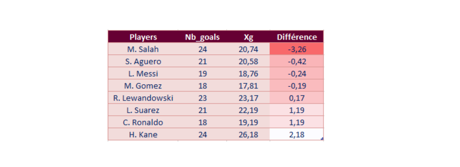
The Expected Goals give us a lot of information about the individual performance of players, especially strickers. By looking at the difference between the xG and the number of goals a player puts in, we can deduce who is the best striker. With the data for the 2017-2018 season we get :

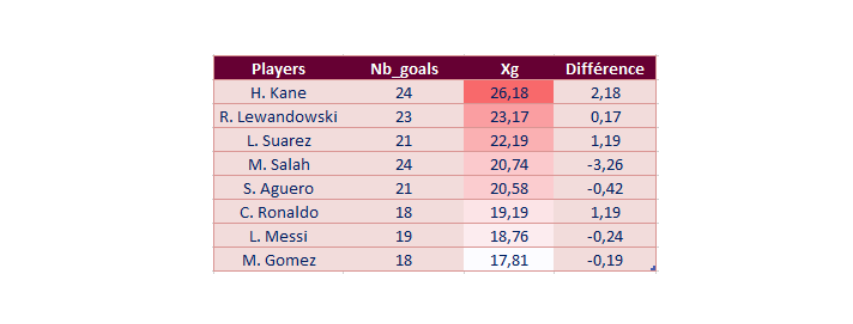
Sorting the xG in descending order, we can know who creates the most situations likely to be converted into a goal:

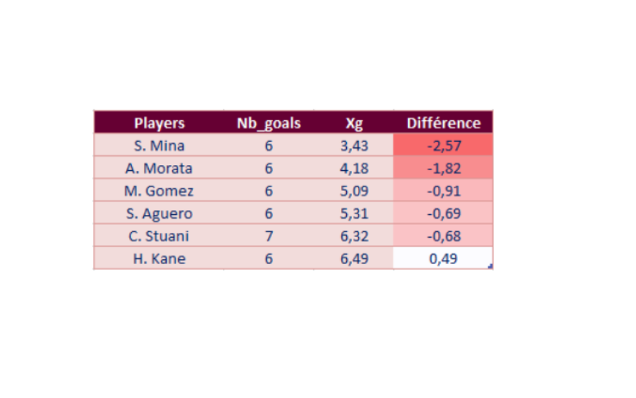
One can also find the best player according to the part of the body (head/right/left) or the best shooter by far. Let's look at the best head shooters:

 To go even further, we can also look at the passers who created the most chances (and thus Expected Goals):

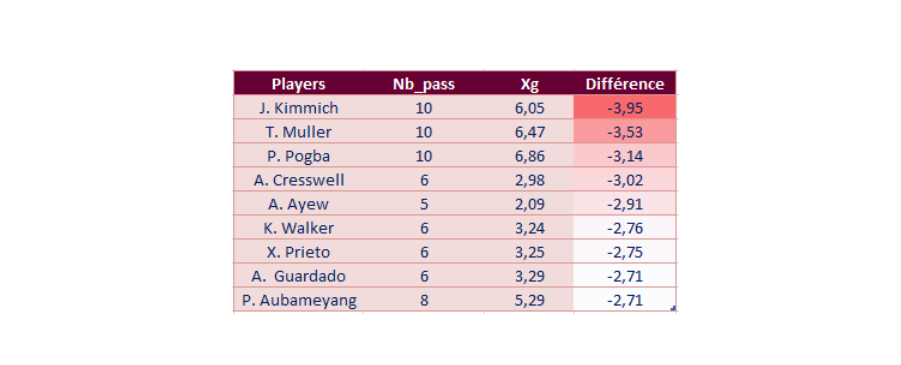
The results make sense and we have a lot of great players at the top of our rankings. It is possible to identify trends and analyze the performance of players. However, the xG model for individual performance has its limitations, especially the predictive aspect where it is difficult to establish consistency.
Still, one of the most common uses of such a model is indeed for prediction. This indicator can also be valuable at a team level. We can calculate the xG "for", the number of goals the team should have scored, and the xG "against", the number of goals the team should have conceded. From this it is possible to model the shape of a team, its luck or bad luck. Obviously if we apply this method on the scale of one or more championships, and model the offensive and defensive performance of each team, we could then predict the outcome of future games and even potentially the outcome of a championship. It may seem puzzling but this metric, which is still relatively new and unperfect, could be an empowering asset.

[1] https://datascience.sia-partners.com/fr/blog/lintelligence-artificielle…
[4] https://medium.com/opex-analytics/why-you-need-to-understand-the-trade-…

Contact : david.martineau@sia-partners.com