Human Intelligence & Artificial Intelligence
Optimization is mostly used to plan and implement organizations, another less known application is that it can also be very effective as a real-time decision making tool to recover from unpredictable disruptions. Here is an example with the container shipping industry.

Maritime transport is a complex industry that binds suppliers and their customers worldwide through the transport of containers over a highly optimized distribution network. These companies operate freight transport networks from one point to another around the world, using large capacity vessels called container ships. In the 1960s, the innovation of containerization had a huge impact on the industry and revolutionized the import-export market of goods by drastically reducing costs, through the increase in the quantity of goods transported per trip.
Today, almost all maritime trade is carried out this way and it is therefore obvious that digitalized solutions associated with mathematical modeling are emerging and mainly focus on this aspect, as economic and environmental gains are easily obtainable and measurable.
First, such a transport system requires goods to be grouped in containers and loaded on large capacity vessels. Secondly, ships and containers travel on a network of shipping routes operated by shipping companies and commercial ports. In most cases, a container's journey from its origin to its destination consists of several consecutive vessels allowing it to reach the final delivery point. The process of loading and unloading containers from one vessel to another is known as transshipment.
One of the most critical problems that shipping companies face on a daily basis and which has never been automated before is the recovery management of unpredictable disruptions. This generates a large amount of extra operational cost. Unpredictable disruption occurs when one or more vessels are delayed. These disruptive events are very hard to predict in the long term (strikes, storms, outages, etc...), resulting in significant deviations from the operational network planning. Not only the delayed vessel is concerned, but also a significative number of adjacent vessels in the network are affected by domino effect, resulting from the delayed transshipments at the ports following the disruption. Meeting delivery deadlines for these goods is therefore directly impacted and represents a threat for the company in terms of customer satisfaction and market share loss to more punctual competitors.
It can be complex for a human eye to identify, with short notice, the best solution given the complexity of the network in place. The longer the operator waits to make a decision, the fewer possibility remains and the higher the catch-up costs. It is crucial for the transport operator to take fast measures to limit the damage to their services caused these services disruptions. This is where operational research, also known as mathematical optimization, comes in. Network modeling of potential recovery actions in a graph structure allows operators to rely on a non-subjective and mathematical tool that gives quantified results in a short period of time. This paper presents the mathematical model developed and applied to the practical cases to guide the shipping company to recover from unpredictable disruptions impacting its network.
Several solutions exist to limit the impact due to service disruption, such as shortening dock time or even inserting an idle vessel waiting at dockside to retrieve waiting containers, but the most common solutions are as follows, it will be these that the model will consider:
The model must take into account the spatial (a vessel sailing between different ports to deliver its goods) and temporal (schedule to be respected under penalty of missing its connection to a container) dimension of the problem.
A first way to model the problem is as a graph and to consider ships, containers and ports as objects defining this graph. Each node in the graph is defined as the possible position of a vessel, in a given port, at a given time. Each arc then represents a possible journey between two port calls (position in a port at a specific time) at a given speed.
How to recover from a disruption and bring all the ships back to the initial schedule while reducing the operational costs and respecting physical constraints. First, a framework must be established, every delay impacting a specific vessel includes a subset of adjacent vessels likely to be affected by the disruption. These adjacent vessels are expected to support the transshipment of delayed containers following the disruption. The scope is then defined geographically around the vessels concerned, their positions and possible routes, and finally by a defined time horizon forcing the vessels to recover before a certain fixed deadline. (As an example, there is a mandatory grouped passage schedule for many companies’ ships through the Suez Canal in order to reduce tax costs). This framework delimits the complexity and reduces the model size to what is really affected by disruptions.
The model is therefore based on a directed time graph where the nodes are associated with a triplet (ship, port, time) and the arcs define the achievable segments of all potential vessel routes through the network according to the recovery scenario.
With the exception of the initial and final nodes, which are fixed by initial conditions and time horizon constraints, all the other nodes have multiple time values because they represent navigation solutions at different speeds and on different routes (due to omitting or skipping port recovery options). All this defines a directed weighted time space graph representing a liner shipping network. Under this simple modeling, there are as many independent subgraphs as there are vessels. The aim is to find the shortest route for all the ships considered.
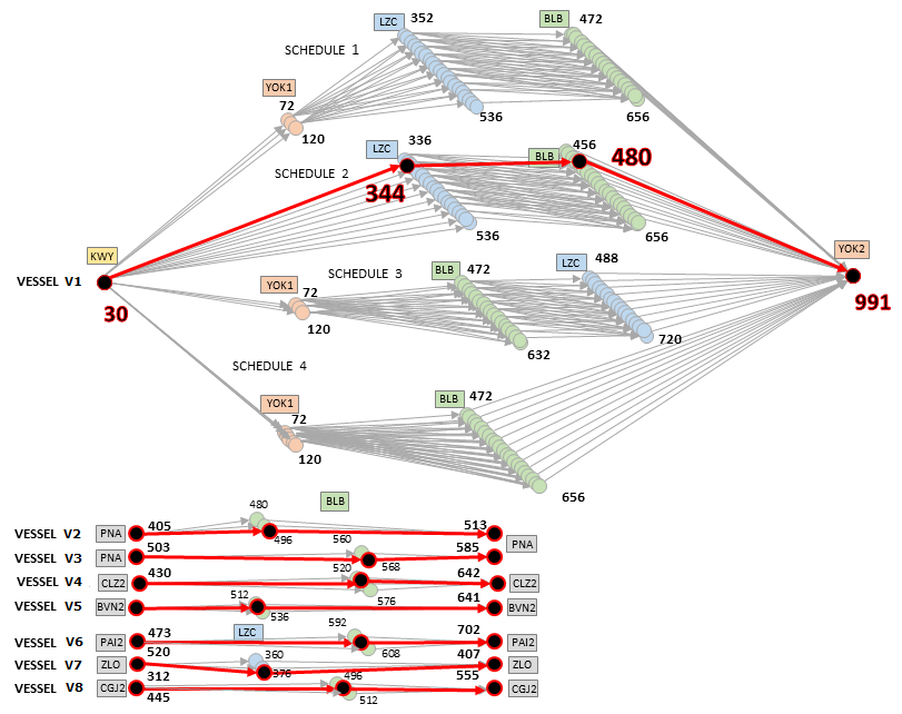
Figure 1: Case of the delay of vessel "V1". In red are represented the optimal solutions identified by the model: Jump from port YOK1 and acceleration of the boat on its way to the final port YOK2
Note to the reader: in this configuration, the choice was made to duplicate some nodes with different scenarios (In Figure 1, the node (V1,LZC,352) for example exists for scenario 1 and 2, and the node (V1,LZC,536) for scenarios 1,2 and 3). This choice is questionable because of the increase in the number of variables to be considered by the mathematical model later, but it also allows not to impose a scenario constraint within the model as no arc links the nodes with different scenarios. This significantly reduce the number of constraints to be considered. It is this second option that has been prioritized in the graph definition.
After the graph network definition, the most important step is to determine the costs and therefore the objective function of the problem that the model will seek to minimize. The idea of using Operational Research is to help solve a complex decision-making problem between the main costs involved:
This model presents good results and has proved its effectiveness on many concrete cases where the model provides a solution at least as good as the one taken by the operators when the situation occurred directly. However, it has many flaws, the most obvious of which is the case of the recovery of containers that have been delayed or missed their connections. Indeed, the current model does not allow to regenerate a schedule for containers that have been delayed or disconnected, they are simply considered as a penalty within the objective function and vanish from the model without having any recovery proposal. It is therefore obvious that graph modeling must integrate a new instance into its modeling: containers.
As described above, the objective function of the problem models the sum of the costs of the solution to be minimized. It takes into account fuel costs and fictitious penalty costs in the event of delay or poor connection of the cargo. The modeled instances are subject to constraints ensuring the feasibility of the generated solution:
The main disadvantage of the previous modeling is that it does not take into account container rerouting. In other words, when a container is seriously delayed or, worse, misses a connection, the model assumes that it will not be delivered and takes it out of the model with an associated cost penalty. No recovery option is envisaged to have it delivered, whereas in reality it will not be abandoned but loaded on another ship and will follow an unplanned journey to its final destination. One could therefore legitimately expect that an optimization tool would incorporate this functionality. The following model addresses this issue.
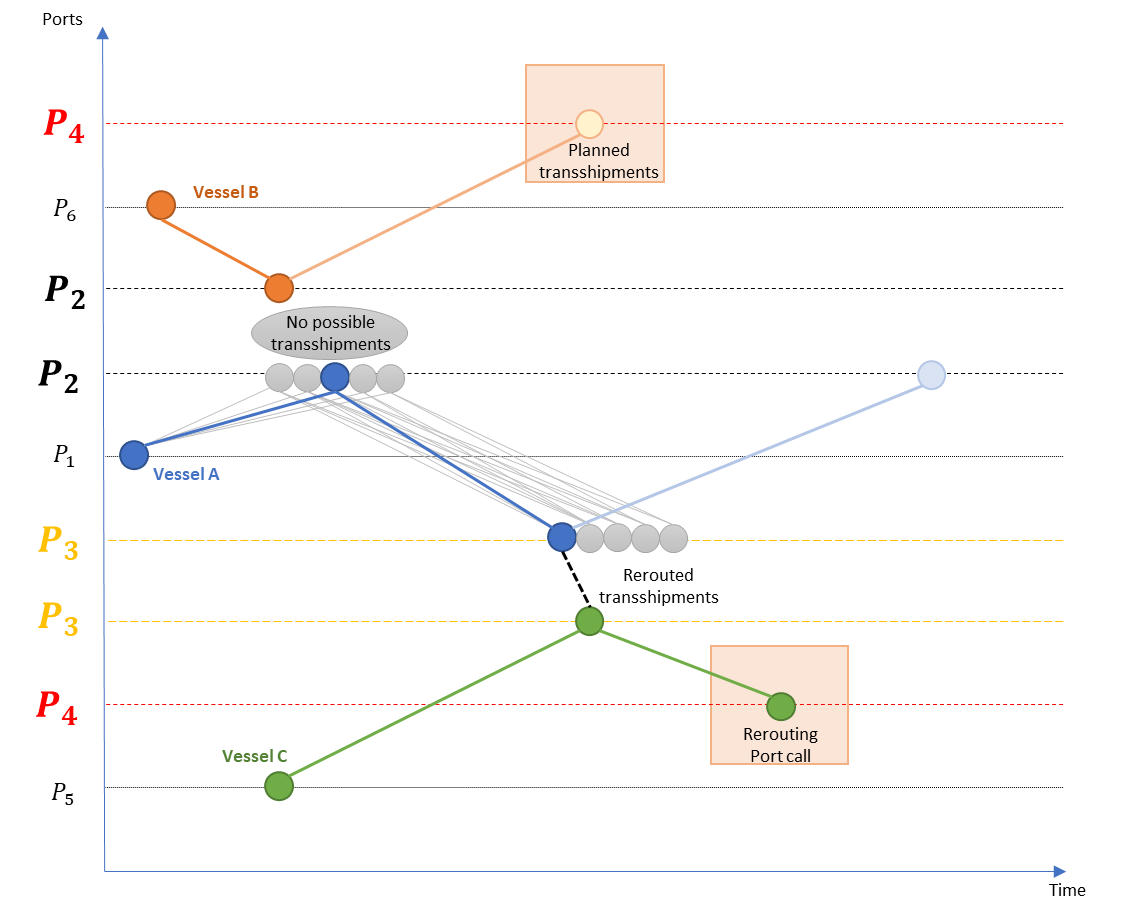
Figure 2: An example of container rerouting. Vessel A has been delayed and is unable to transship at port P2, so it is accelerating to port P3 with vessel C and delivering the containers to port P4, late but at the right destination.
In order to model containers as objects within the network, we had to adapt the shape of our graph. Different additional arcs and nodes have been created for the containers to integrate their particular spatial displacement characteristics into the graph network. Containers are no longer considered as objects linked to vessels, but as objects, free to move from one ship to another provided that both vessels call at the same port and the first before the second. Containers also enter the network through gate nodes connected to the first and last port calls (which are fixed and known). Non-connection arcs are also created, between these "gate" nodes, these are weighted with the cost of the wrong connection connecting these door nodes for each group of containers. All these new features of the graph add complexity to the problem as both vessel and container flows are processed in parallel. This is a so-called Multi-flow optimization problem.
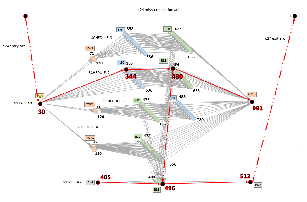
Figure 3: Case of vessel "V1" with a single group of containers "c24". In red are represented the optimal solutions identified by the model with the solid arcs representing the vessel’s routing and in dotted line the group of containers c24 considered
The algorithms of both models were run for each of the four use cases. The solutions and performances were compared and confronted with the actual decisions that had been taken by an operational staff. First of all, it should be mentioned that both models provided solutions at least as good as those chosen by the operators on situation. For some, the decisions made by agents were optimal according to the model, for others, the use of both models would have made it possible to better advise agents and save planning recovery expenses. The two models provided the same solutions for all four use cases since there was no room for cargo rerouting in either use case. In order to evaluate the performance of the new model, the method of selecting ships to be included in the simulation must be rethought to add vessels capable of proposing alternative routes for delayed containers and better evaluate cargo rerouting solutions.
During this study, another use case was developed to test the potential benefits of integrating container rerouting. Based on the cases used for the first model, the data has been enlarged by adding additional vessels offering alternative routes for containers to reach their final destination. The results have been satisfactory since the second model modeling containers proposes to redirect some of them, while the first model considers them simply as delayed or unconnected containers. The second model has proved to be satisfactory in proposing better results than the first one, on the condition that a broader network is considered by the model, so that all possible recovery actions for ships and containers are fully evaluated.
Operations Research serves here as a powerful decision-making accelerator, all modelled options are evaluated and compared analytically on their estimated costs and the optimum is highlighted. This method remains a powerful tool for data processing considering input parameters and is not intended to replace the decisions of a human operator. The latter can then more precisely evaluate the feasibility of a theoretical optimal solution proposed by the tool and iteratively change the settings according to his observations in order to take the best decision possible.
This study is based on the work of Alexandre Orhan and Florian Binter on disruption management in liner shipping.
If you want to know more about our AI solutions, check out our Heka website
Contact : david.martineau@sia-partners.com

